- 수강한 강의
: Ch03.sklearn-전처리 기본-07.Standardization(표준화) / Ch04.sklearn-분류-01.iris 데이터 로드 (dataset 활용) / Ch04.sklearn-분류-02.dataset으로부터 데이터프레임 만들기 / Ch04.sklearn-분류-03.데이터의 불균형 (imbalance) 그리고 stratify 옵션 / Ch04.sklearn-분류-04.logistic regression (로지스틱 회귀) / Ch04.sklearn-분류-05.모델 선언, 학습(fit), 예측(predict) 프로세스
오늘은 전처리의 표준화와, sklearn 분류에서 iris 데이터 로드(dataset 활용), dataset으로부터 데이터프레임 만들기, 데이터의 불균형 (imbalance) 그리고 stratify 옵션, logistic regression, 모델 선언, 학습 (fit), 예측 (predict) 프로세스에 관하여 작성해보겠습니다.
Ch03.sklearn-전처리 기본-07.Standardization(표준화)
표준화는 평균이 0과 표준편차 1이 되도록 변환 해주는 것이다.표준화를 실행시키기 위해서는 다음과 같이 StandardScaler를 import 시켜준 다음에 특정 변수에 StandardScaler() 함수를 지정해서 표준화를 실행한다. 그러고 난 다음에 샘플데이터를 생성해준다.from sklearn.preprocessing import StandardScaler standard_scaler = StandardScaler() x = np.arange(10) # outlier 추가 x[9] = 10009번째 인덱스에 1000이라는 값으로 변경한다. 1000으로 변경한 이유는 기본 0~9까지의 데이터를 가지고 하게 되면 평범한 값의 평균과 표준편차등이 나오기 때문에 따로 outlier를 지정해서 평균값을 올리기 위해서 1000으로 변경한 것이다.
그리고 만들어진 데이터를 토대로 평균값과 표준편차를 구해준다.
x.mean(), x.std()(103.6, 298.8100399919654)scaled = standard_scaler.fit_transform(x.reshape(-1,1)) scaled.mean(), scaled.std()(4.4408920985006264e-17, 1.0)
scaled라는 변수에 위에 저장한 standard_scaler에 fit_transform을 활용하여 x변수를 저장해준다.
그러고 scaled의 평균값과 표준편차를 확인해본다.round(scaled.mean(), 2), scaled.std()(0.0, 1.0)
그러면 다음과 같은 결과값이 나오게 되면서 평균값이 0으로 맞춰지고, 표준편차는 1로 맞춰진것을 확인할 수 있다.
다음과 같은 결과값이 나오게 된다. 하지만 다음 값을 보기에는 편하지가 않다. 그래서 보기 좋게 scaled의 평균값에 round() 함수를 사용하여 보기 편하게 설정해 준다.Ch04.sklearn-분류-01.iris 데이터 로드 (dataset 활용)
우선 불필요한 경고 출력을 방지하기 위해서 다음과 같은 코드를 실행 시켜준다.그러고 pandas를 import 실행시켜준다.
import warnings # 불필요한 경고 출력을 방지합니다. warnings.filterwarnings('ignore') import pandas as pd다음은 sklearn.dataset에서 제공해주는 다양한 샘플 데이터를 자세하게 명시해준 사이트이다.
iris 데이터셋
다음은 실습으로 사용할 iris 데이터셋에 설명이 나와있는 사이트이다.from sklearn.datasets import load_iris # iris 데이터셋을 로드합니다. iris = load_iris()iris 데이터셋을 실행시키기 위해서 다음 코드를 먼저 실행시켜준다.다음의 데이터 셋은 딕셔너리 형식을 되어있다.
다음 데이터 셋의 내용은 다음과 같다.
- DESCR: 데이터셋의 정보를 보여줍니다. - data: feature data. - feature\_names: feature data의 컬럼 이름 - target: label data (수치형) - target\_names: label의 이름 (문자형)print(iris['DESCR'])예시로 DESCR의 값을 출력해본다.
  ```
  #.. _iris_dataset:
  #Iris plants dataset
  #--------------------
  #**Data Set Characteristics:**
    :Number of Instances: 150 (50 in each of three classes)
    :Number of Attributes: 4 numeric, predictive attributes and the class
    :Attribute Information:
        - sepal length in cm
        - sepal width in cm
        - petal length in cm
        - petal width in cm
        - class:
                - Iris-Setosa
                - Iris-Versicolour
                - Iris-Virginica
    :Summary Statistics:
    ============== ==== ==== ======= ===== ====================
                    Min  Max   Mean    SD   Class Correlation
    ============== ==== ==== ======= ===== ====================
    sepal length:   4.3  7.9   5.84   0.83    0.7826
    sepal width:    2.0  4.4   3.05   0.43   -0.4194
    petal length:   1.0  6.9   3.76   1.76    0.9490  (high!)
    petal width:    0.1  2.5   1.20   0.76    0.9565  (high!)
    ============== ==== ==== ======= ===== ====================

    :Missing Attribute Values: None
    :Class Distribution: 33.3% for each of 3 classes.
    :Creator: R.A. Fisher
    :Donor: Michael Marshall (MARSHALL%PLU@io.arc.nasa.gov)
    :Date: July, 1988
  The famous Iris database, first used by Sir R.A. Fisher. The dataset is taken
  from Fisher's paper. Note that it's the same as in R, but not as in the UCI
  Machine Learning Repository, which has two wrong data points.
  This is perhaps the best known database to be found in the
  pattern recognition literature.  Fisher's paper is a classic in the field and
  is referenced frequently to this day.  (See Duda & Hart, for example.)  The
  data set contains 3 classes of 50 instances each, where each class refers to a
  type of iris plant.  One class is linearly separable from the other 2; the
  latter are NOT linearly separable from each other.
  .. topic:: References
   - Fisher, R.A. "The use of multiple measurements in taxonomic problems"
     Annual Eugenics, 7, Part II, 179-188 (1936); also in "Contributions to
     Mathematical Statistics" (John Wiley, NY, 1950).
   - Duda, R.O., & Hart, P.E. (1973) Pattern Classification and Scene Analysis.
     (Q327.D83) John Wiley & Sons.  ISBN 0-471-22361-1.  See page 218.
   - Dasarathy, B.V. (1980) "Nosing Around the Neighborhood: A New System
     Structure and Classification Rule for Recognition in Partially Exposed
     Environments".  IEEE Transactions on Pattern Analysis and Machine
     Intelligence, Vol. PAMI-2, No. 1, 67-71.
   - Gates, G.W. (1972) "The Reduced Nearest Neighbor Rule".  IEEE Transactions
     on Information Theory, May 1972, 431-433.
   - See also: 1988 MLC Proceedings, 54-64.  Cheeseman et al"s AUTOCLASS II
     conceptual clustering system finds 3 classes in the data.
   - Many, many more ...
   ```
다음은 iris['DESCR']인 iris 데이터셋의 정보를 출력한 것이다.
data = iris['data'] data[:5]array([[5.1, 3.5, 1.4, 0.2], [4.9, 3. , 1.4, 0.2], [4.7, 3.2, 1.3, 0.2], [4.6, 3.1, 1.5, 0.2], [5. , 3.6, 1.4, 0.2]])feature_names = iris['feature_names'] feature_names['sepal length (cm)' , 'sepal width (cm)', 'petal length (cm)' , 'petal width (cm)']
다음의 값은 iris 데이터 셋에서 data 값 중에서 속성값을 출력한 결과 값이다.다음은 iris 데이터 셋의 feature_names 값에 대한 결과값이다.
     - sepal : 꽃 받침
  - petal : 꽃잎
target = iris['target'] target[:5]array([0, 0, 0, 0, 0])
다음은 iris 데이터 셋의 'target'의 최상위 5개 값을 출력한 것이다.iris['target_names']array(['setosa', 'versicolor', 'virginica'], dtype='<U10')
다음은 iris 데이터셋의 label의 이름을 출력한 것이다.Ch04.sklearn-분류-02.dataset으로부터 데이터프레임 만들기
위에서 로드한 데이터셋인 iris 데이터셋을 데이터프레임으로 만들어보겠습니다. 데이터셋을 데이터프레임으로 만들기 위해서는 pandas의 DataFrame 함수를 활용하면 된다.```python df_iris = pd.DataFrame(data, columns=feature_names) df_iris.head() ``` ``` sepal length (cm) sepal width (cm) petal length (cm) petal width (cm) 0 5.1 3.5 1.4 0.2 1 4.9 3.0 1.4 0.2 2 4.7 3.2 1.3 0.2 3 4.6 3.1 1.5 0.2 4 5.0 3.6 1.4 0.2 ```위에서 작성된 data를 df_iris 변수에 데이터 프레임으로 만들은 다음에 작성된 데이터 프레임의 최상위 5개 항목에 대해서 확인하는 과정이다. 작성된 데이터 프레임을 보게 되면 'sepal length (cm)', 'sepal width (cm)', 'petal length (cm)', 'petal width (cm)'의 항목들이 컬럼으로 작성되고 그에 해당하는 값들이 작성된 것을 확인할 수 있다.
      df_iris['target'] = target
  df_iris.head()
sepal length (cm) sepal width (cm) petal length (cm) petal width (cm) target 0 5.1 3.5 1.4 0.2 0 1 4.9 3.0 1.4 0.2 0 2 4.7 3.2 1.3 0.2 0 3 4.6 3.1 1.5 0.2 0 4 5.0 3.6 1.4 0.2 0다음은 iris 데이터셋에 존재하는 target 정보를 df_iris 데이터 프레임의 target의 컬럼명의 value값으로 추가하고, 정보가 제대로 추가되었는지 확인하는 절차이다.
다음은 iris 데이터셋을 시각화한 것이다.
데이터를 시각화하기 위해서는 matplotlib과 seaborn을 import 해준다.import가 끝나면 seaborn을 활용하여 scatterplot을 그리면 된다.import matplotlib.pyplot as plt import seaborn as sns sns.scatterplot('sepal width (cm)', 'sepal length (cm)', hue='target', palette='muted', data=df_iris) plt.title('Sepal') plt.show()
다음 그래프는 df_iris 데이터셋에 존재하는 target 값들의 분포를 산점도로 표현을 한 것이다. 코드 중에서 hue='target' 옵션이 존재하게 된다. 다음의 옵션은 우리가 scatter로 표현하고자 하는 값인 target 컬럼의 데이터를 서로 다른 색으로 표현하게 해주는 옵션이다. 최종 결과 그래프를 봐도 target의 값들인 0, 1, 2인 값들에 따라서 색들이 다르게 표현된 것을 확인할 수 있다.

다음은 df_iris에서 petal과 관련된 항목 중에서 target의 값들을 산점도(scatter) 그래프로 출력한 것이다. 작성 방법은 위와 동일하다.from mpl_toolkits.mplot3d import Axes3D from sklearn.decomposition import PCA fig = plt.figure(figsize=(8, 6)) ax = Axes3D(fig, elev=-150, azim=110) X_reduced = PCA(n_components=3).fit_transform(df_iris.drop('target', 1)) ax.scatter(X_reduced[:, 0], X_reduced[:, 1], X_reduced[:, 2], c=df_iris['target'], cmap=plt.cm.Set1, edgecolor='k', s=40) ax.set_title("Iris 3D") ax.set_xlabel("x") ax.w_xaxis.set_ticklabels([]) ax.set_ylabel("y") ax.w_yaxis.set_ticklabels([]) ax.set_zlabel("z") ax.w_zaxis.set_ticklabels([]) plt.show()
다음은 df_iris 데이터 프레임을 3D 형식으로 나타내서 출력한 것이다. 여기서Axes3D(fig, elev=-150, azim=110)값이 있다. 이것은 3D로 만들는데 전체적인 크기는 fig변수에 저장한 크기로 하고 elev은 입면뷰각에 해당하는 값이고, azim은 방위각, 시야각에 해당하는 값이다. 그리고 PCA(n_components=3) 이라는 옵션값이 존재한다. 이것은 기존 df_iris 데이터셋에 존재하는 성분 값을 조정해주는 것이다. 3D에 경우에는 표현할 수 있는 축의 값이 3개 존재한다. 하지만 df_iris 데이터셋에는 4개의 성분 값이 존재하게 된다. 따라서 이러한 4개의 성분 값을 주성분에 해당하는 3개의 성분을 추출하여 표현하기 위해서 사용한 옵션이다.Ch04.sklearn-분류-03.데이터의 불균형 (imbalance) 그리고 stratify 옵션
다음은 데이터셋의 불균형에 대하여 작성 해보겠습니다.
우선 df_iris 데이터셋을 활용하여 train과 test의 데이터를 나누고 나눠진 값을 맞게 나눠졌는지 확인하고, seaborn을 활용하여 y_train의 값이 얼마나 되는지 출력해본다.from sklearn.model_selection import train_test_split x_train, x_valid, y_train, y_valid = train_test_split(df_iris.drop('target', 1), df_iris['target']) x_train.shape, y_train.shape((112, 4), (112,))x_valid.shape, y_valid.shape
((38, 4), (38,))sns.countplot(y_train)

다음의 값은 다시 실행할 때마다 값이 다르게 나오게 된다. 우선 사진의 값을 보게 되면 0, 1, 2에 해당하는 값들이 불균형 적으로 나온 것을 확인할 수 있다. 그래서 이러한 것을 균형적으로 맞춰주기 위해서 stratify옵션을 사용하면 target의 값을 균형적으로 맞춰서 출력할 수 있다. 사용하는 방법은 다음과 같다.x_train, x_valid, y_train, y_valid = train_test_split(df_iris.drop('target', 1), df_iris['target'], stratify=df_iris['target']) sns.countplot(y_train)``` 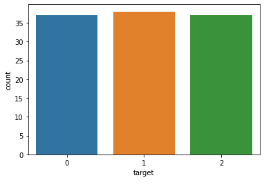 다음 사진을 보게 되면 target에 해당하는 0, 1, 2에 해당하는 값이 균형있게 출력된 것을 확인할 수 있다. ```python x_train.shape, y_train.shape((112, 4), (112,))x_valid.shape, y_valid.shape((38, 4), (38,))
stratify를 활용한 후에 각 train인과 valid의 모양을 확인해보면 stratify 사용하기 전과 동일한 모양임을 확인할 수 있다.Ch04.sklearn-분류-04.logistic regression (로지스틱 회귀)
다음은 로지스틱 회귀에 관한 자세히 설명한 사이트이다.
logistic regression다음은 로지스틱 회귀에 관한 인터넷 검색 내용이다.
- 로지스틱 회귀(영어: logistic regression)는 영국의 통계학자인 D. R. Cox가 1958년에 제안한 확률 모델
- 독립 변수의 선형 결합을 이용하여 사건의 발생 가능성을 예측하는데 사용되는 통계 기법
LogisticRegression, 서포트 벡터 머신 (SVM) 과 같은 알고리즘은 이진 분류(2개의 클래스를 말하는 것)만 가능합니다. (2개의 클래스 판별만 가능합니다.)
하지만, 3개 이상의 클래스에 대한 판별을 진행하는 경우, 다음과 같은 전략으로 판별하게 됩니다.
one-vs-rest (OvR): K 개의 클래스가 존재할 때, 1개의 클래스를 제외한 다른 클래스를 K개 만들어, 각각의 이진 분류에 대한 확률을 구하고, 총합을 통해 최종 클래스를 판별
one-vs-one (OvO): 4개의 계절을 구분하는 클래스가 존재한다고 가정했을 때, 0vs1, 0vs2, 0vs3, ... , 2vs3 까지 NX(N-1)/2 개의 분류기를 만들어 가장 많이 양성으로 선택된 클래스를 판별
대부분 OvsR 전략을 선호합니다.Ch04.sklearn-분류-05.모델 선언, 학습(fit), 예측(predict) 프로세스
모델 선언과 학습, 예측하기 위해서는 다음 코드를 작성하면 된다.from sklearn.linear_model import LogisticRegression model = LogisticRegression() # 모델 선언 model.fit(x_train, y_train) # 모델 학습LogisticRegression(C=1.0, class_weight=None, dual=False, fit_intercept=True, intercept_scaling=1, l1_ratio=None, max_iter=100, multi_class='auto', n_jobs=None, penalty='l2', random_state=None, solver='lbfgs', tol=0.0001, verbose=0, warm_start=False)prediction = model.predict(x_valid) # 예측 prediction[:5]array([2, 0, 0, 2, 1])(prediction == y_valid).mean()1
다음의 코드들이 모델 선언, 모델 학습, 예측, 평가에 관한 코드 들이다. 그리고 최종적으로 평가를 해서 나온 값이 1이 나오게 되는데 다음의 값은 앞에서 stratify옵션을 추가해서 나오게 되는 값이다. 하지만 이러한 stratify 옵션을 제거하고 평가를 하게 되면 나오는 값은 달라지게 된다.(prediction == y_valid).mean()0.9473684210526315
다음과 같은 결과값이 위에서 stratify옵션을 제거하고, 모델 선언, 모델 학습, 예측, 평가한 최종 결과값이 되게 된다.
이렇게 전처리의 표준화와, sklearn 분류에서 iris 데이터 로드(dataset 활용), dataset으로부터 데이터프레임 만들기, 데이터의 불균형 (imbalance) 그리고 stratify 옵션, logistic regression, 모델 선언, 학습 (fit), 예측 (predict) 프로세스에 관하여 작성해보았습니다.
- 데이터 분석
- 홈페이지에서 강의 찾는 방법
패스트 캠퍼스 -> 온라인 -> 올인원 패키지 -> [데이터 분석 강의 보러 가기] -> 직장인을 위한 파이썬 데이터 분석 올인원 패키지 Online.
패스트 캠퍼스 - [데이터 사이언스] 직장인을 위한 파이썬 데이터 분석
직장인을 위한 파이썬 데이터 분석 올인원 패키지 Online
'데이터 분석' 카테고리의 다른 글
| [패스트 캠퍼스 수강 후기] 직장인을 위한 파이썬 데이터 분석 올인원 패키지 Online 22일차 (0) | 2021.04.26 |
|---|---|
| [패스트 캠퍼스 수강 후기] 직장인을 위한 파이썬 데이터 분석 올인원 패키지 Online 21일차 (0) | 2021.04.20 |
| [패스트 캠퍼스 수강 후기] 직장인을 위한 파이썬 데이터 분석 올인원 패키지 Online 19일차 (0) | 2021.04.13 |
| [패스트 캠퍼스 수강 후기] 직장인을 위한 파이썬 데이터 분석 올인원 패키지 Online 18일차 (0) | 2021.04.12 |
| [패스트 캠퍼스 수강 후기] 직장인을 위한 파이썬 데이터 분석 올인원 패키지 Online 17일차 (0) | 2021.04.06 |


댓글